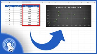
Printable Scatter Chart: A Quick Guide to Creating and Using Them
A scatter chart is a powerful way to display the relationship between two quantitative variables. When you need to present your data in a clean, print‑ready format, a printable scatter chart is essential. This article walks you through the basics of creating a scatter chart, adding quadrants, fitting a line of best fit, and exporting the final graphic for high‑quality printing.
Why Choose a Printable Scatter Chart?
Printable scatter charts are ideal for:
- Academic presentations and research papers
- Business reports and executive summaries
- Classroom worksheets and handouts
- Data‑driven posters and infographics
Because the data points are plotted directly on a Cartesian plane, they allow quick visual assessment of trends, clusters, and outliers. When you print the chart, you can embed it in documents, slide decks, or even print multiple copies for classroom use.
Step‑by‑Step: Creating a Simple Scatter Chart in Excel
Below is a concise workflow that mirrors the “quick and easy video tutorial” style many learners prefer. The same steps apply whether you’re using Excel, Google Sheets, or another spreadsheet application.
- Prepare Your Data
- Organize your independent variable in column A and dependent variable in column B.
- Label the first row with descriptive headers (e.g., “Hours Studied” and “Test Score”).
- Select the Data
- Click and drag to highlight the two columns of data.
- Insert Scatter Chart
- Navigate to Insert → Charts → Scatter (X, Y) or Bubble Chart → Scatter with only Markers.
- Excel will create a basic scatter plot with default axes.
- Format for Print
- Click on the chart area and choose Format Chart Area. Set a white background and adjust the border to a thin gray line.
- Increase the font size of axis titles and tick labels to at least 10 pt for readability when printed.
- Add a chart title and subtitle using the Chart Title box.
- Add Quadrants (Optional)
- Insert a reference line at the mean of each axis: right‑click on the horizontal axis → Add Data Label → Series Options → Show as a line. Repeat for the vertical axis.
- Use the Shape Tools to draw a light‑gray rectangle that represents each quadrant.
- Draw a Line of Best Fit
- Select the data series, then Chart Design → Add Chart Element → Trendline → Linear.
- Choose Display Equation on Chart and Display R